


In this article we show how to prepare historical files with continues features and a discrete target for an ensemble of securities using DLPAL PRO. Then, we apply machine learning on a random sample of half of the data and test the results on the remaining half. The results are promising since the quality of generated features is high.
Data generation and preparation
The most important step in any machine leaning application is gathering data and generating relevant features with an appropriate target class. Although most work is usually focused on the use of algorithms, generating the proper data is more of an art and where the actual edge is found.
In a nutshell, to use machine learning a data file is required with a sufficient number of rows (instances) and columns that correspond to attributes. In trading applications, the simplest form of machine learning involves a group of continuous attributes and a discrete attribute for the target. The attributes (features predictors, etc.) can be values of technical indicators and fundamental data. The target is usually a binary class of the next period return in the timeframe under consideration. The objective is to determine the probability of the sign of the returns. Then, we can rank predictions according to objectives. But without the proper attributes, this is an exercise in futility.
One advantage of DLPAL PRO is that it generates features based on the proprietary p-indicator. These features are unique and offer opportunities for identification of price action anomalies. In Part One, we presented feature generation for a single security. In this article, we use features generated from a group of securities and specifically from historical data of D0w-30 stocks.
We select data for Dow-30 stocks since 01/2000 and we create a file with 500 instances (rows) of features using DLPAL PRO’s P-Indicator history tool, as shown below:
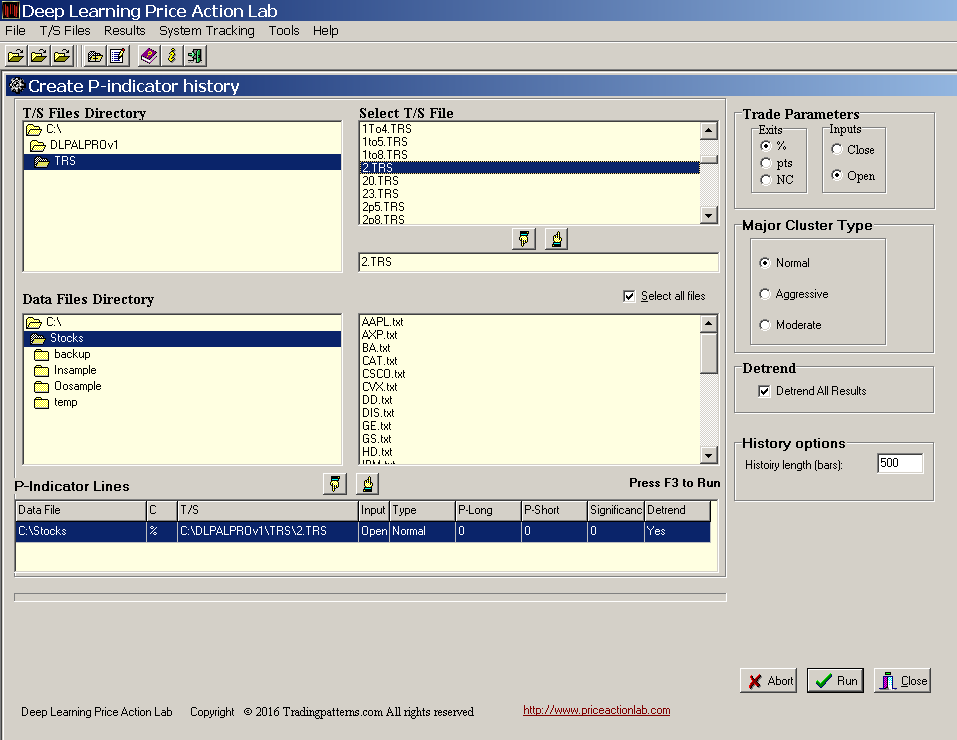
We used percent exits of 2%, entry at the open, a Normal cluster and the detrend option for the feature calculation. It took the program a few hours to generate the history file due to the enormous amount of calculations involved.
We then combine the generated file with features and historical data for SPY. This is how the file looks like:
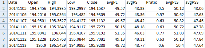
There are five features: avgPL, avgPS, Pratio, avgPLS, avgPSS. We employ some feature engineering to reduce these to three by taking the difference of the first two and last two, since it represents the directional bias. We also add a target based on two day returns. This is how the resulting file looks like:
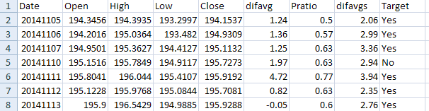
We use the 2-day return because we know from experience that features from ensembles of securities predict returns two days in the future. This is where experience comes into play. However, we will also use machine leaning to determine if this experience is biased.
Training and testing
The objective of supervised machine learning is to determine the probability of class “Yes”. We start with binary logistic regression and we randomly sample 50% of the instances to use in training and the remaining 50% to use for testing. Below is the confusion matrix from the training sample:
| Yes | No | Sum | |
| Yes | 82 | 45 | 127 |
| No | 60 | 61 | 121 |
| Sum | 142 | 106 | 248 |
The error rate is 0.4234. Next we are interested in the error in the test set. The confusion matrix is shown below:
| Yes | No | Sum | |
| Yes | 81 | 70 | 151 |
| No | 47 | 50 | 97 |
| Sum | 128 | 120 | 248 |
The test sample error rate is 0.4718.
We next train the classifier in the whole sample and then use bootstrap to determine the average test set error. This comes out to 0.4522. We can then conclude that there is some prediction potential with this simple classifier.
We also used Support Vector Machines with RBF Kernel on the whole sample and then bootstrap. The resulting average test set error was 0.4343. The results look promising and we can proceed with backtesting.
We implement the logistic function in Amibroker with the coefficients calculated from the training sample. The backtest for the combined sample is shown below:
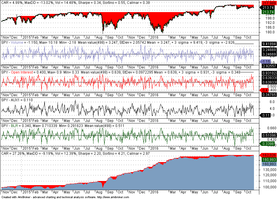
In the above chart, Volume is difavg, open interest is Pratio and AUX1 is difavgs. The logistic function BLR is also shown. In a period from 11/05/2014 to 10/26/2016, CAR is 27.3%, net return is 61%, max DD is -9.2%, the win rate is 59% and profit factor is 1.82. The stop is two bars after the open and all positions are at the open. Commission of $0.01 per share was used and equity was fully invested.
Of course, half of the backtest is on training data but sampling was random to reduce bias. Although this is not a strategy that can be used in actual trading, the results show that the concept is promising but additional work is required to get to the stage where there is something usable. However, the ability of DLPAL PRO to generate unique features provides a good starting point.
If you have any questions or comments, happy to connect on Twitter: @priceactionlab
You can download a demo of DLPAL from this link.