We present in this article a novel strategy based on features generated by DLPAL LS software in the weekly time frame that trades long/short 85 large cap stocks from the S&P 100 universe and combines buy and hold, trend-following, position and short term trading.
The usual paradigm in trading strategy development involves differentiating buying and holding securities from timing strategies, such as trend-following, position and short-term trading. The strategy in this article presents a novel paradigm where all these different styles of trading arise from the same algorithm and are naturally combined to generate the end result.
Buy and hold strategies
The main advantage of buy and hold strategies is minimization of transaction cost. The main disadvantage is that they cannot deal with a large drawdown and as a result risk-adjusted returns are usually lower than those of effective timing strategies.
Trend-following strategies
Trend-following attempts to maximize returns by squeezing as much profit as possible from price trends. The main disadvantage of these strategies is lower performance during sideways markets that can even erase gains from long uptrends.
Position and short-term strategies
Timing price action is difficult due to noise but if done properly it can offer a high win rate and profit factor at low exposure to price action. The main disadvantage is increased transaction cost that in some cases is a large portion of realized profit.
A novel approach
Combining buy and hold, trend-following and position/short-term trading can be done with naive approaches that integrate related strategies but in the case of the strategy presented in the article, this combination arises naturally from the application of the same algo. The key is in generating features that facilitate the combination. This is done by DLPAL LS software, which offers unique ways of dealing with price action.
Data preparation
For strategy development we used weekly adjusted data of 85 stocks from the S&P 100 universe that have price history going back to year 2000.
Feature engineering
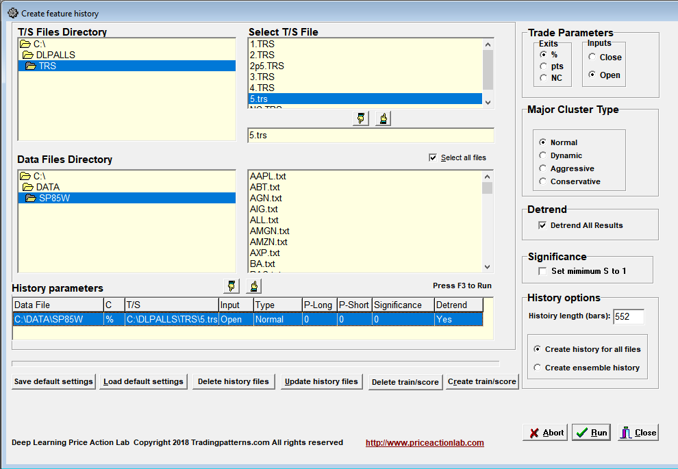
The historical values of the features for each of the 85 stocks were calculated by DLPAL LS software. We used the “Create Features History” option from Tools, as follows:
In the above setup we select the directory with the weekly data for the 85 stocks. We also select a T/S file with 5% profit target and 5% stop-loss for feature classification. This is a reasonable size reward/risk for weekly data.
We also selected the Normal major cluster. The history length is set to 552 bars so that calculation of features will start on 01/04/2008. The data history before that is used in the calculations. The weekly data range from 01/07/2000 to 07/27/2018. There are a total of 960 weekly bars in each file and the first 408 are used to start the feature generation. We also elect to have the results adjusted for trend bias by checking the option “Detrend All Results.”
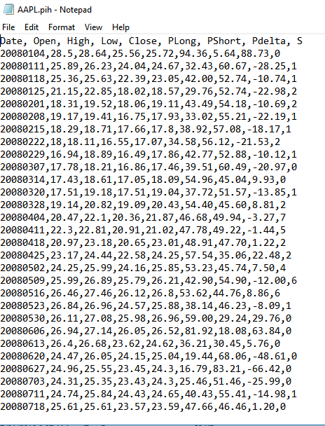
DLPAL LS takes the 85 original historical data files of the stocks as input and creates new files with extension .pih that include the feature values for each instance (row). An example is shown below for AAPL.
PLong and PShort are the long and short directional probabilities, respectively, Pdelta is their difference and S is the significance of the results. These are the four features calculated in this mode of operation of DLPAL LS. There are also other features related to ensembles of securities not used in this article.
Importing results in backtesting program
This is an important step that allows data visualization and to make sure everything worked as expected. The generated .pih files for each stock are imported in Amibroker in separate database. We use Amibroker because of the ease of importing historical data with additional fields. The four indicators are imported as follows: PLong is assigned to Volume, PShort is assigned to Open Interest, Pdelta is assigned to Aux1 and S to Aux2. An example chart of a stock with the indicators is shown below. The chart also included the product Aux1*Aux2, corresponding to Pdelta*S, because this is what is used in the strategy as an entry/exit rule.
Defining and backtesting the strategy
Specifications
Time-frame: Weekly (adjusted data)
Strategy type: Long/short, exit and reverse
Universe: 85 stocks from S&P 100 index
Backtest period: 01/04/2008 – 07/27/2018
Features calculation period: 01/07/2000 – 12/27/2007
Maximum open positions: 84
Position size per stock: Equity/84
Position entry and exit: Open of next bar
Commission per share: $0.01
Strategy logic
Buy if AUX1 × AUX2 > 100 (this is equivalent to Pdelta × S > 100
Short if AUX1 × AUX2 < -100 (this is equivalent to Pdelta × S < -100
We use a bias of +/- 100 to limit the number of trades and reduce commission cost. The bias results in longer holding periods for positions.
Strategy performance
| Parameter | Strategy | SPY TR B&H |
| CAGR | +4.05% | +8.7% |
| Max. DD | -5.4% | -52% |
| Sharpe | 0.36 | 0.43 |
| MAR | 0.74 | 0.17 |
| 2008 | -1.4% | -34% |
| 2011 | +1.4% | +2.5% |
MAR (CAGR/Max. DD) for the strategy is 0.74 versus 0.17 for SPY total return in the same period. The strategy has low drawdown and can be leveraged to generate returns in excess of SPY total return but at a much lower drawdown.
Below are the equity curve, underwater equity curve, and results of a Monte Carlo simulation. (Click on images to enlarge.)
 |
 |
 |
The simulation indicates that there is less 5% probability of a drawdown that exceeds 16%.
Distribution of trades holding period
Below is a cumulative distribution of trade holding period for the above strategy:
It may be seen that 80% of the trades have holding period of less than 30 weeks, about 66% of the trades have holding period of less than 18 weeks and 25% of the trades last two weeks, which is the minimum since the exit bar is considered part of the holding period.
These are the symbols where buy and hold since 2008 was applied by the strategy: MMM, SPG, KO, RTN, MO, GD. For these symbols there has been only an entry to open a long position and no other signals. This is the buy-and-hold part.
Weekly Execution
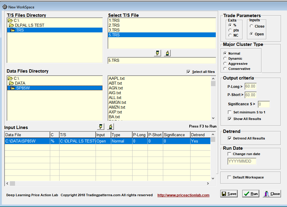
Weekly execution involves updating all data files and ranking stocks according to Pdelta*S score. This is done in DLPAL LS with a few clicks. An example as of 07/27/2018 is shown below. First the workspace used:
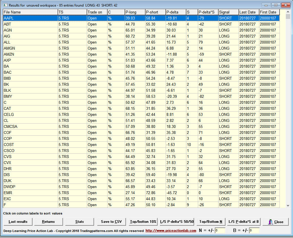
Below are the raw results:
Below are the results ranked according to Pdelta*S score and filtered for bias B > +100 and < -100. This only takes a few seconds:
Alternatively, the features can be updated automatically after updating data files and the model can generate the signals so that filtering and visual inspection is not required.
Feature updating
Features can be updated automatically from “Create Feature History” tool. In addition, train and score files can be generated for use with machine leaning classifiers. Some users of DLPAL LS prefer to let classifiers identify an abstract model and make the final selection of stocks to trade. Support Vector Machines (SVM) or even Binary Logistic Regression (BLS) can be used for this purpose. Additional features of choice can be added by the user to the files for more sophisticated models.
Click here for more details of how hedge funds can order a free fully-functional demo of DLPAL LS to test for a month.
If you have any questions or comments, happy to connect on Twitter: @priceactionlab
Strategy performance results are hypothetical. Please read the Disclaimer and Terms and Conditions.


