
There are widespread misconceptions about quant trading even by those who use it in hedge funds. In this article we expose some of these misconceptions and we offer a practical example.
A recent article in Bloomberg titled “Computer Models Won’t Beat the Stock Market Any Time Soon” demonstrates the level of misconception about quant models in the hedge fund industry (See reference at the end.)
1. Fundamentals still rule
Most hedge funds, even in equity long/short space, still use fundamental analysis. I have worked with some of them and I have run across people in key positions who know little or even nothing about backtesting that is at the core of quantitative analysis. Anyone who tries to transition to quantitative trading from fundamentals will face a steep learning curve. Hiring a physicist who knows well quantum mechanics often does not solve the problem and in some cases it makes it worse. During a conference I met a mechanical engineer with a PhD who was fresh in quantitative trading and was all excited about applying fluid dynamics concepts to price analysis. I told him this was done already in the 90s with no success. This is what everyone should remember:
The smartest individuals in physics and math may look stupid when involved with financial markets. Quant trading is a practitioners field and the learning curve is about 10 years or even longer. You just do not apply Heisenberg’s Uncertainty Principle to markets and make it big. It is foolish to expect that.
2. Quant trading is difficult because data is non-stationary
If data were stationary, then markets would be too efficient to trade and no one would make profit to cover cost anyway. It is the non-stationarity that provides the profit and also makes forecasting difficult. Non-stationarity makes quant trading difficult by ruling out naive models based on attempts to treat markets as stationary, which is a prerequisite of most traditional forecasting methods. If you do not have an approach to quant trading that is compatible with non-stationarity, do not complain about it, try to deal with it.
3. Signals-to-noise ratio is very small
That did not stop a trivial forecasting method to outperform the market for many years during a period when economists were touting the efficient market hypothesis. The proof is in this article.
When you hear someone talking about “signal-to-noise ratio”, ask them how they measure it. Most do not even know and just repeat what they have heard on financial television at some time claimed by someone who also heard it somewhere.
4. Edge is small
It is interesting how many in the industry do not understand the difference between edge and hit rate, or win rate. The win rate is the edge when the payoff ratio is 1. If the payoff ratio is not 1, then the expectation must be used. For example, if the win rate is 60% and payoff is 1, then the edge is 20%, which comes from 60-(100-60). But if the payoff is 0.5 at 60% win rate, then the edge is 0.5 × 60 -(100-60) = -10%, i.e., there is no edge but an expected loss. Those that confuse the win rate for the edge when payoff is less than 0.67 are going to lose anyway since the expectation is negative. This has happened to some hedge funds after a large loss that erased many months or years of gains and caused the payoff ratio to decrease despite of the win rate staying high. This is the story: one large loss does not impact much the hit rate but may reduce substantially the payoff ratio to erase the edge.
But this is not the end of the story; quants do not look for small edges because there are no large ones. Our data-mining algos identify large edges on a daily basis in a variety of markets. The problem with large edges is that the sample size is usually smaller and in many cases tiny. This makes the analysis of the significance of these larger edges difficult or impossible. On the other hand, small edges turn out to have larger samples. This is one, and the main in our opinion reason, that quants focus on small edges. But in order to fully comprehend these details you need a lot of skin-in-the-game. Even when the details are revealed that is not enough. The whole procedure of identifying and validating edges is complex. Most will be happy to skip it and just draw a line on a chart.
5. People in analysis usually have no idea what hedge fund traders do
Why some funds employ hundreds of PhDs is really curious since they are not needed. These funds need experienced practitioners, such as ex pit traders or NYSE specialists, most with just high school diploma, and even people with skin in the game in various business sectors. One may be compelled to think that the wealthy and successful fund operators exercise some kind of social policy to employ PhDs that otherwise would be forced to compete for tenure under harsh conditions no different in principle from those in Survivor reality shows.
In fact, no one knows the final decisions of traders and it is also hard to relate them to holdings of funds if they are disclosed. I found that out when I worked for a hedge fund and by error I received some trade confirmations from the broker. The trader was essentially fading the signals of one of the fund’s own analysts. As I found out lateral the fund operator liked to also hire what he thought were consistent losers. Those losers may offer some type of an edge for a while. Most PhDs that come from fields unrelated to finance may turn out to be consistent losers.
This summarizes a few misconceptions we often read in popular finance articles. Below is a practical example, which the reader may skip if not interested in details.
An example
We use DLPAL S to identify strategy edges in SPY ETF with 53% or higher hit rate. We also require 100 or more trades per strategy in the in-sample, 1.5 or greater profit factor and less than 10 consecutive losers. Trades are entered at the open of next bar. The in-sample for identification is daily data from 01/29/2993 to 12/31/2009. The out-of-sample for validation is from 01/03/2010 to 05/24/2019.
The first step is to determine the smallest possible profit target and stop-loss to evaluate strategy performance. This is done below using the in-sample data.
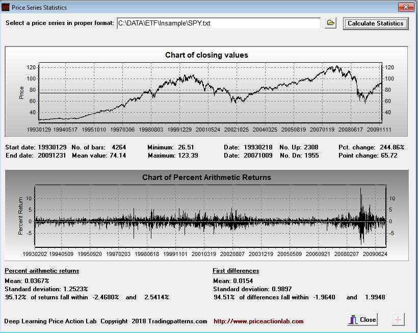
Since 95.12% of all daily returns fall within -2.47% and +2.54%, we elect to use 2.5% for both profit target and stop loss. In this way the stop-loss is slightly outside the range and the profit target is slightly inside it.
Below is the DLPAL S workspace used for the identification.

The results are shown below:
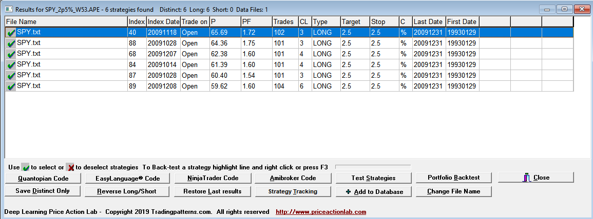
Each line in the results is a strategy that satisfies the performance parameters specified on the search workspace. Index and Index Date are used internally. Trade on is the entry point, in this case the Open of next bar. P is the success rate of the strategy, PF is the profit factor, Trades is the number of historical trades, CL is the maximum number of consecutive losers, Type is LONG for long strategies and SHORT for short strategies, Target is the profit target, Stop is the stop-loss and C indicates whether % or points for the exits, in this case it is %. Last Date and First Date are the last and first date in the data file.
DLPAL S found six long strategies in the in-sample that fulfilled the parameters specified on the workspace. The highest win rate is less than 66% and the lowest is a little more than 59%.
DLPAL S can generate code for a variety of platforms to backtest a strategy that combines any selected strategies from the results with OR Boolean operator. In this case we select all strategies, we generate the code and then copy and paste it in Amibroker. Below are the results for the out-of-sample only.
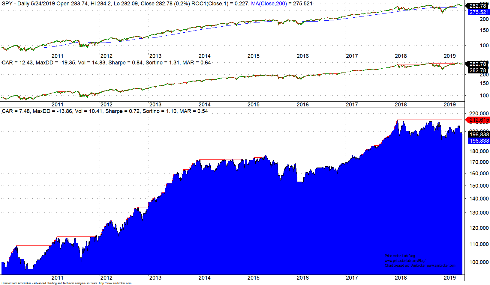
Performance as measured by Sharpe is at about 85% of buy and hold (shown in middle chart.) This is good out-of-sample performance that shows robustness of the edges. But as already mentioned, the hit rate of the edges in the in-sample did not exceed 66%. In order to increase the hit rate, the trade sample requirement would have to be lowered. There are ways of validating strategies with smaller samples but this is beyond the scope of this article.
Another serious misconception of quant traders
The in-sample/out-of-sample testing is used to validate the data-mining method primarily. You do not have to and actually should not use a model identified in the in-sample in actual forward trading since during its identification it was not exposed to a variety of new market conditions. But identifying a new one on the whole data sample may not be good practice if the predictors are not correlated and the model is different. The advantage of using DLPAL S is that the predictors are correlated and the data-mining bias is minimum although never zero. Most GP and NN algos will create a new model unrelated to the in-sample model when exposed to the whole price history. This is one reason that their developers insist on using the model identified in in-sample. But this is the wrong approach when the predictors used (indicators, factors, features, etc.) are unrelated in the two models, the in-sample and the one in the whole sample. The bias can be reduced in data-mining algos that use well-defined predictors by selecting only a specific group but in abstract models such as NN it cannot be reduced.
There are several other misconceptions about quant strategies and their development but here we only referenced a few key ones.
Reference
Computer Models Won’t Beat the Stock Market Any Time Soon
If you found this article interesting, I invite you follow this blog via any of the methods below.
Subscribe via RSS or Email, or follow us on Twitter
If you have any questions or comments, happy to connect on Twitter: @mikeharrisNY