

Highly curve-fitted strategies are common in financial blogosphere. The usual objective of the developers of such strategies is to impress their audience with exceptional performance and gain an advantage over competition. Those not aware of the mechanics of strategy development may be impacted most.
Most quants are aware of the tricks that one can use to generate high returns in backtests, especially of large cap trading strategies. But some with lack of experience may think: “The strategy is trading a large universe of stocks; therefore the numbers must be real.”
False, it is actually the reverse: the larger the universe, the most effective some of the tricks used for data-mining and p-hacking.
The main reason is this: the larger the universe, the higher the possibility of finding a few exceptional winners in the past to curve fit the performance of the strategy. Will comparable winners be available in the future? No one can answer this question.
Main curve-fitting mechanisms
- Momentum ranking (example: rate-of-change over a lookback period.)
- Moving average crosses (usually daily or monthly.)
- Various filters to eliminate previous bear markets (often moving average crossovers.)
- Trailing stops to curve-fit on past performance.
Popular equity universes used in curve-fitting
- S&P 100, S&P 500
- NASDAQ-100
- Russell 1000, 2000, 3000
Optimized parameters
Below is a list of parameters that are often used to optimize performance.
- Number of long (short) positions.
- Ranking score lookback (rate-of-change period, RSI period, etc.)
- Buy (short), sell (cover) conditions and their parameters.
- Trailing stop percentage or number of exit bars.
- Lookback periods used on various filters.
With a large number of parameters available to a backtesting program in conjunction with a large universe of securities, anything is possible in backtests.
An explosive mix
The mix of curve-fitting mechanisms with large stock universes and many optimized parameters is explosive. With the use of optimization, high annualized returns can be realized in backtests at “seemingly acceptable” levels of risk. But past performance is in most cases the result of curve-fitting on market conditions that may never repeat in the future.
Fitted, curve-fitted and genuine strategies
All strategies are fitted one way or another on historical data. The curve-fitted strategies are those that are more prone to fail when there is even a slight change in market conditions. The genuine strategies instead identify presence of market anomalies that have positive expectation.
For example, a moving average crossover is not an anomaly but a condition that attempts to identify an anomaly. If the anomaly is not present, the result is a loss. This often occurs during sideways markets.
Buying a number of stocks that rank at the top according to some measure and selling those at the bottom is not an anomaly but an attempt to take advantage of a possible anomaly provided it is there in the first place.
A large parameter space allows developers to “create” artificial anomalies that are specific to the values of parameters used and historical conditions. But in the future, a slight change in market conditions may require a different set of parameters to achieve even an acceptable result. In a nutshell, this is the problem of optimization in trading strategy design.
For the backtests in this article we used Norgate data that include current and past constituents to remove survivorship bias. We highly recommend this data service to those who would like to remove survivoship bias from backtests (we do not have a referral arrangement with the company.)

This is a long/short strategy that trades large cap stocks. The developer uses it to attract customers for trading strategy design services. Below is the equity curve with statistics, monthly returns and a drawdown profile.
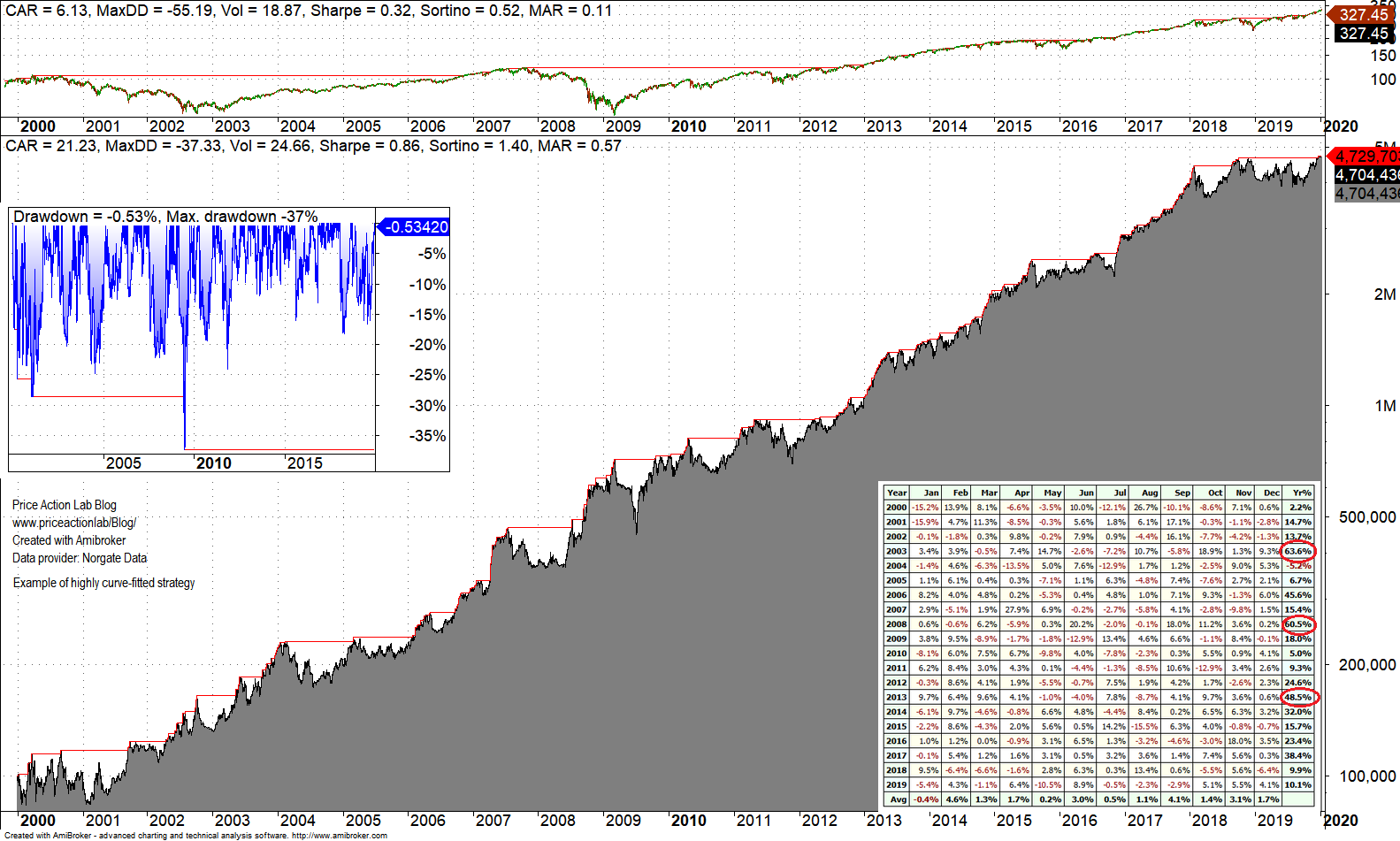
The effort to optimize the equity curve is evident to experienced quants. Optimized parameter set maximizes returns for certain years to provide equity curve jumps.
This particular strategy has about 10 parameters that were optimized! A key parameter is the number of traded long and short securities. Below is a graph that shows how the annualized return, which is 21.23% for the equity curve above, varies as a function of number of long (short) positions. All the other parameters were kept constant.
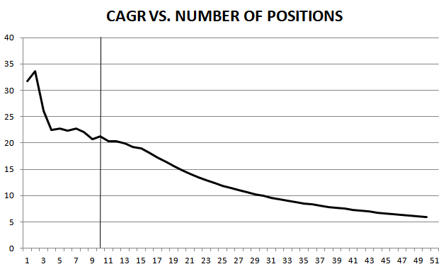
The above graph shows that the ranking mechanism and associated conditions were optimized to detect the stocks with the largest gain in the past. For 1 -3 open positions the strategy generated an annualized return of nearly 35%. This means that a $10M account would have grown to nearly $200M in the last 10 years! In comparison, in the last ten years $10M invested in SPY ETF would have grown to $35M. The huge outperformance must come from somewhere but it is not clear how. Even with the 10 long (short) positions and annualized return of 21.3%, the account would have grown to about $70M.
It may be seen from the above graph that as the number of open long(short) positions increases above 30, the annualized return gets close to market performance as the results of the curve-fit start to fade. The key with these strategies is to select the best trade-off of parameters to maximize returns while keeping the maximum drawdown as low as possible. Below is a graph of the maximum drawdown as a function of open positions.
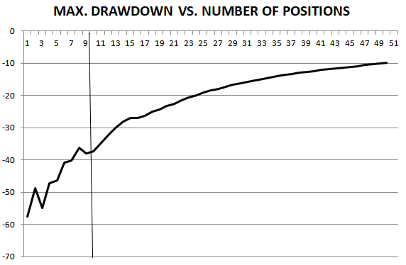
Near 8 open positions, there is a local maximum. Then, there is a local minimum near 10 and afterwards the maximum drawdown decreases steadily. The local maximum and minimum points are often used in optimized parameter selection.
In order to get the drawdown below 20%, about 25 open positions must be held and that reduces the annualized return (CAGR) near 8% rather than the optimized 21.3%. The choice of the developer to optimize the annualized return is to offer the impression of a highly profitable strategy. But if the maximum drawdown of the market (SPY) is matched in the last 10 years, the strategy must underperform the market total return of about 13.5% by a wide margin. It appears then there is a conscious decision to maximize return at the expense of maximum drawdown.
Example 2
This is a long-only strategy for trading large cap stocks. The developer attempts to impress prospective customers of similar strategies with a high annualized return the bulk of which comes from two years due to optimization on a limited sample starting in 2007, as shown in the chart below.
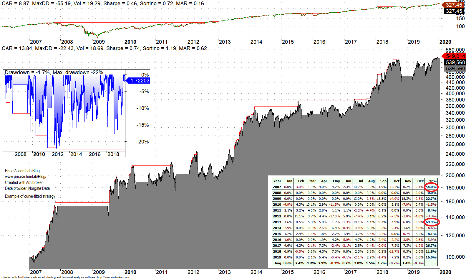
Needless to say that we tested this strategy on an extended sample and it generated unacceptable drawdown.
This strategy has fewer parameters, only three, but since it does not have a short leg it is easier to optimize on data from mostly bull market since the 2008 bear market is filtered out.
Below is a graph that shows how the annualized return, which is 13.8% on the above chart, varies as a function of long number of positions. All the other parameters were kept constant.
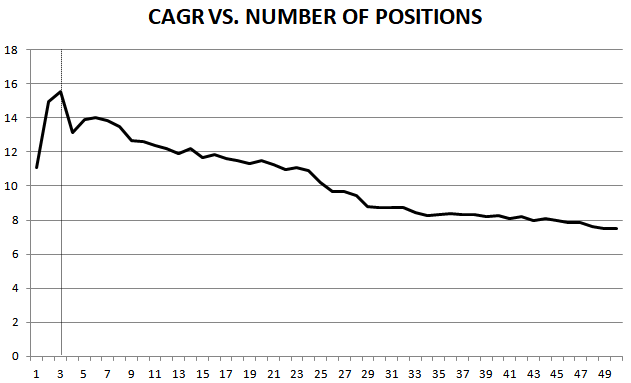
It is immediately seen that the developer chose a number a little higher than the global maximum at 3. The graph of maximum drawdown as a function of open positions clearly shows the reason for this choice.
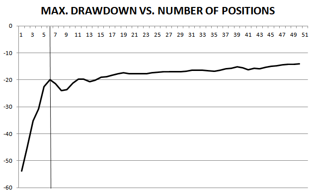
For 3 open positions the maximum drawdown is too high but drops fast and makes a local minimum near 5 positions. Then it starts decreasing monotonically but along with it also CAGR decreases.
In the particular case the developer is lucky because the maximum drawdown is close to -20% near the CAGR global maximum.
This is a case of a less severe curve-fit but one that relies on filtering out bear markets. As a result this particular strategy can stay out of the market for extended periods of time. Also, in case market conditions persist, there is chance of this strategy working well in the future but if they change, the losses can be devastating depending on rate of change.
Conclusion
Developers of trading strategies that have realistic performance and avoid curve-fitting as much as possible have to fight ludicrous claims by some developers that hit the optimization button and select the best and most impressive result. Most experienced quants can immediately spot optimize strategies but this is not always the case with aspiring hedge fund managers and other non-quant types. In this article we provided some details of the mechanism of curve-fitting and two examples of curve-fitted strategies.
Charting and backtesting program: Amibroker
Data provider: Norgate Data
Technical and quantitative analysis of major stock indexes and 34 popular ETFs are included in our Weekly Premium Reports. Market signals for position traders are offered by our premium Market Signals service
If you found this article interesting, you may follow this blog via RSS or Email, or in Twitter